Activity 3: Scilab Basics

In this activity, we learn the basics of Scilab-- sort of a free version of Matlab. Here we learned how to generate arrays of numbers (using linspace()) and N-dimensional matrices (using the ndgrid() function) and eventually used them to generate different shapes i.e. circle, square, corrugated roof, gratings along some direction x or y, annulus(doughnut-shaped figure), circular aperture with gaussian transparency (Whoa there!); ellipse; and the cross.

Figure 1. Centered Circle with corresponding Scinote script.

In the manual[1], we were first introduced to the different operations that can be done in Scilab. As practice, we were to execute the sample code shown in Figure 1 and the result was a centered circle. I was a little bit bothered by its unsharp edges so I tried a larger value for $nx$ and $ny$ which determines the number of points. I tried $nx = ny = 1000$ and got the following:

Figure 2. Tried nx = ny = 1000 because I was bothered by the blurred edge. I like this better and will be using this value for the next images I will be generating.

Seeing that Maam Jing has provided the essential stuff that I will be needing to generate shapes, what's left for me was to change one or two lines in the code.

First off, the Centered Square Aperture.

Figure 3. Centered Square Aperture

This one's easy. I guess everyone knows what makes a square, a square. All its sides are equal! So I used the $abs( )$ function that will give me both positive x and y values (less than 0.7 as I set it). Line 7 says I want to make all points less than 0.7 to be white (value of 1).

Next, the Corrugated Roof.

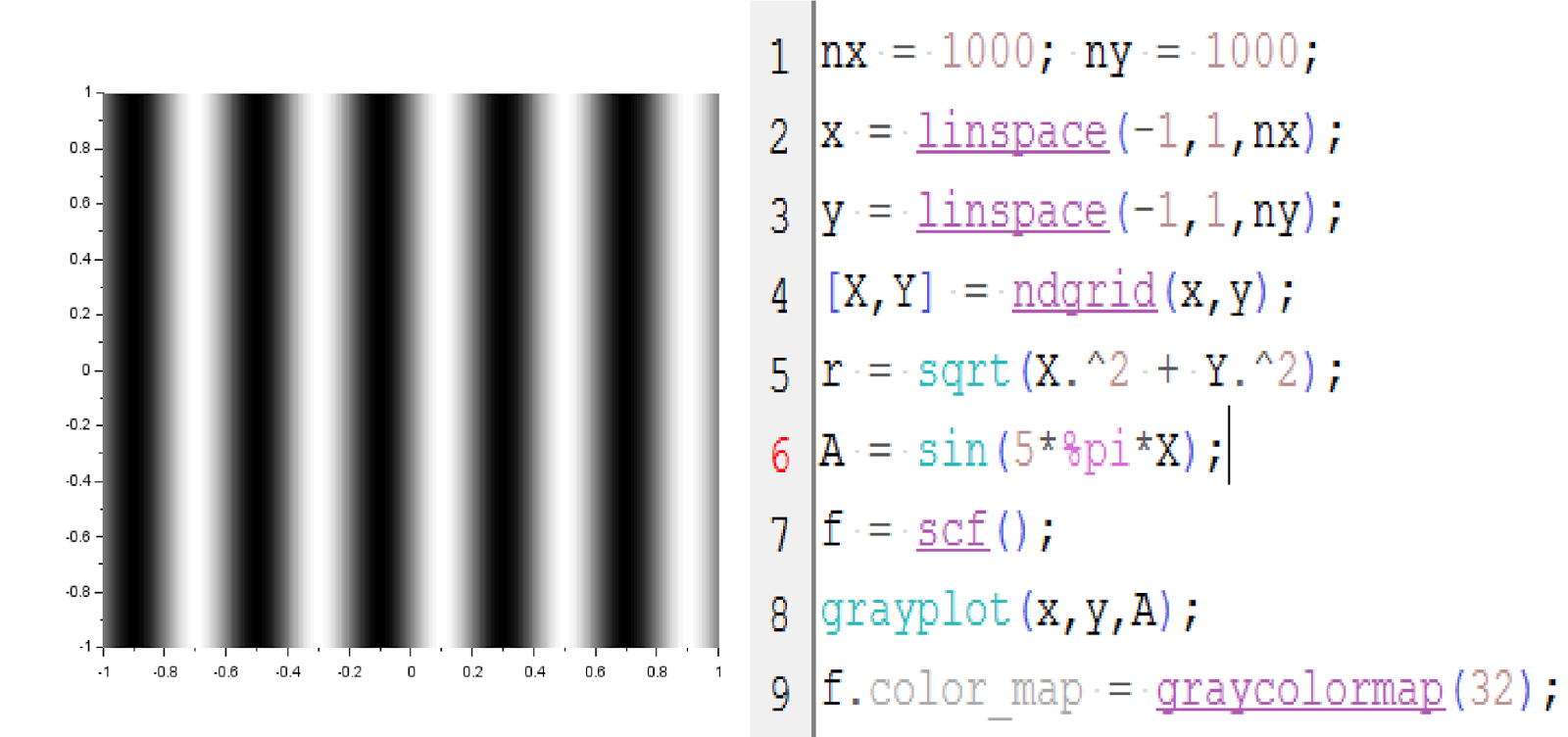Figure 4. Corrugated Roof

At first, I thought we were asked to draw a roof -- the triangular one we see on our houses. Haha And I was a little bit intimidated. Maybe because of the word corrugated huhu. Then I realized, since we are only dealing with 2D objects, we are actually only asked to draw the surface of the material being used for the roof. (Whooo !Nabunutan ako ng tinik :D ). So when we look at the edge of our roofs, we see a wave pattern so I thought, "yes, maybe it's a wave function!". I checked Google and I was right. Tadaaaa! One thing I noticed here is that the image is actually just a series of alternating black and white only that the transition in color is not sharp. It has gradient! So maybe, since we have a gradient, we also have values in between black ( px value = 0) and white (px value = 1). What I imagined looking at this plot is that, the bright spots are the portions on the roof that is being lit by the sun while the dark ones are the depressions that are overshadowed by the adjacent groove. :))

The next image is another repetitive pattern so I thought of using another wave function. This time I used the squarewave() function in Scilab.

Figure 5. Gratings along x-direction

We were asked to create gratings along the x-direction. As we know, square waves have two amplitude values over time and space and that is 0 and some amplitude value A. I used this property to draw a pattern whose pixel values are binary [0- black grating, 1- white grating]. As I increase the $nx$ and $ny$ the number of gratings increase as well.

Figure 6. Annulus

I must admit, I did not know what an annulus is so I had to asked my research tito, Antonino Paguirigan Jr who was also working on something at the same time I was working on this. He said it looks like a doughnut, so I made a doughnut. The annulus is similar to the centered circle only that I had to add an additional condition: $ r > 0.35 = 1$ to make a dark circle in the middle. :)

Figure 7. Circular aperture with Gaussian transparency

I said I was intimidated by corrugated. This time gaussian transparency did a better job. I need mighty Google's guidance! :">  To be able to create a graded transparency that emanates from the center (colored white and has the greatest pixel value) I needed to use the form of a Gaussian function.

 $ f(x)  = ae^{-\frac{(x-b)^2}{2c^2}}$

where I took $a  = \frac{1}{\sqrt{2\pi}}$ and $c =1$ and $(x-b) = 0.3$ is standard deviation or the spread from the center.

I also tried a different value. Let $(x-b) = 0.7$ and I got this.

Figure 8. Trying out different values to see the difference. This is what I got for $(x-b) = 0.7$

Another shape that we have been very much acquainted with during the course of our Physics life is the ellipse which is characterized by the mathematical equation: $\frac{x^2}{a^2} + \frac{y^2}{b^2} = 1 $ where $ a \neq b $ and that whose values decides the major axis of the ellipse.

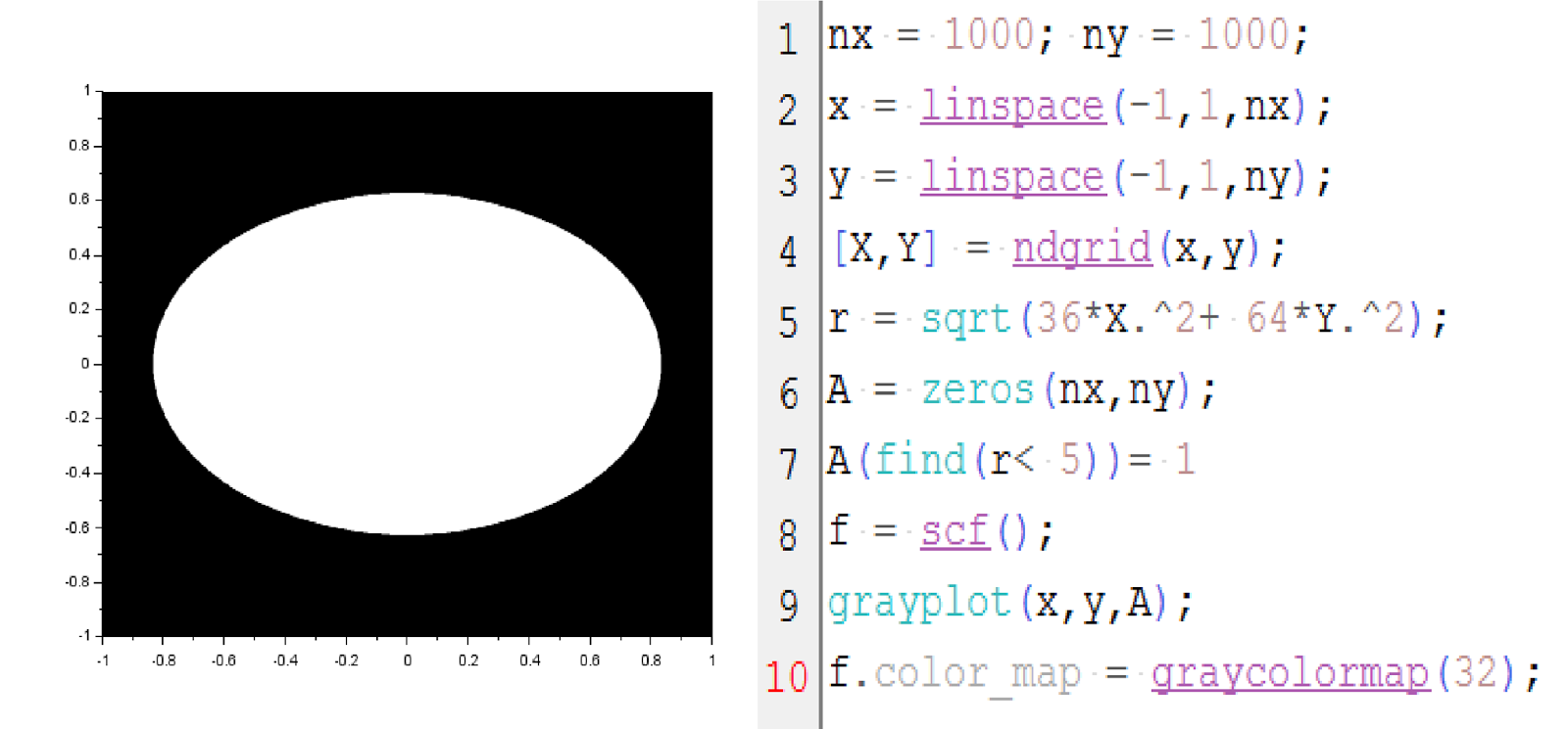Figure 9. Ellipse with X as the major axis.

Lastly, we have the cross.  This one is also similar to making a square aperture but includes additional conditions. But here, instead of using the abs( ) function, I explicitly provided the values just to be sure. ( I was actually tempted to color it red, para red cross! :)) )

Figure 10. Cross

The following figures are some images that I generated by combining different synthetic images. I was a little annoyed by Scilab because when I run my code to display them, it stops. And I discovered that in order to display one image, I had to close and reopen Scilab everytime. Arghhh. I am yet to install another version and see if it works.

Figure 11. Exploration #1: Gaussian + Ellipse, setting region $ r > 0.3 = 1$

Here I combined the ellipse and the Gaussian transparency synthetic images. I imagined the dark spot in the middle to be a black hole and the gradient indicates the radiation field. Well, it's very simplistic and very unelegant compared to the real thing. But it's all in my head so it's fine. :))

Figure 12. Exploration #2: Tried out different trigonometric function, $cos^2 (\pi r^2)$

This time I arbitrarily chose a familiar function $cos^2 (\pi r^2)$ which I expected to give also a familiar wavy form. I was surprised to get saddles which repeats in space. I remembered the logo of the X-factor only that it's blurry. :))

Figure 13. Exploration #3: Gaussian combined with a wave function with frequency $\omega = 5$ 

This time I combined a Gaussian with a sine function with frequency $\omega = 5$ and got five point sources that to me look like Arago spots. But I think since the others are unclear, it's only because of the misalignment in my set-up :D

Finally, I combined a sine wave and a square wave and got the following. Here I employed element-to-element multiplication.

Figure 14. Sine Wave + Square Wave. Element-wise multiplication was also employed.

Over all, this activity has helped me refresh my math and analysis as to how to make the shapes and to not modify the given code too much. And also, I had fun imagining stuff from the images I generated. Please don't judge me po. huhu :D


References:

[1] M. Soriano. "Scilab Basics", Activity Manual. AP186. (2016)

Activity 2: Digital Scanning

In this activity, we aim to reconstruct a digitally scanned hand-drawn plot by using ratio and proportion.

The plot I used was taken from the College of Science Library from the old journals section and was scanned by Ate Lina Galapon of the NIP.( It was my first time to go up to the second floor of the lib. :)) Good opportunity before I graduate! )

Figure 1. Scanned hand-drawn plot from a very old Applied Physics journal in the CS Lib

The image is 834x625 in size. First, I took the coordinates of the graph tick marks. For convenience in identifying the coordinates, I zoomed in through the image (800%). Now that I have the coordinates, what I did was to take the difference between the adjacent ticks to determine the number of pixels corresponding to a unit. Along the x-axis, there is an average of 73 px in between the tick marks and 91 px along the y-axis.

Figure 2. Image dimension and other noted measurements used for removing the translation

Next, we were asked to choose arbitrary points on the plot curve that would help us reconstruct the original one. Since, the origin of an image is at the upper left corner as noted by Patrick Elegado, I needed to adjust the y coordinate of the arbitrary points. To do that, we subtract the y-values from 625. Doing that I got this plot:

Figure 3. Plot of the arbitrary points

 It does not end there. We also needed to remove the translation along both directions by subtracting the number of pixels corresponding to the margin of the plot. Given the origin of the plot to be at (94,572), the $(x,y)_{new} = ( x_coordinate - 94, y_coordinate - 53)$ .

Finally, to get $(x,y)_{actual}$ which is the actual pixel value along x and y after proper scaling we use dimensional analysis.

$X(px) * \frac{1 actual}{73 px} = X(actual)$

$Y(px) * \frac{0.25 actual}{91 px} = Y(actual)$

Now that we have the actual coordinates, we plot them in Excel. In addition, because I want to reconstruct the original plot as close as possible, I also plotted the scatter and their respective error bars.

Figure 4. Reconstruction of the hand-drawn plot

Overall, I had fun doing this activity. Haha I was also able to laugh at how sabaw I am when I consulted Maam Jing about the physical equation part (which in my case is y = mx + b) and then Maam Jing went over to see what I'm doing because I was talking about averaging the slopes between any two of my chosen arbitrary points but huhu Maam came over and showed me how powerful Excel is! Oo nga, may best fit line :) Ayun.

References:
[1] M. Soriano. "A2-Digital Scanning", AP186 Manual.(2016)

Everything Will be Clearer Through This Lens

When I first came to Physics, my notion was that I would be disconnected from the tangible reality and be left in a room pondering over the floating mathematical symbols that the dead geniuses were very much acquainted to. I still cringe at the thought of me not taking a bath because there's something I do not understand. To make the long story short, now that I'm already in my fifth year (and hopefully my final year as an undergraduate), I never thought that Physics would include something as the stuff we do in class i.e. image processing, cameras and programming! To be honest, I do not think I actually understood my Physics 11x series at that time it was taught...I don't think I truly understood the others either. :( Fortunately, my recent Phy 18x subjects made things clearer to me i.e. Physics 121 and Math 121.1 stuff made easier by AP183 (ex. Laplace transforms! Yun pala yun and Fourier series :)) . All those fancy maths and concepts contextualized into something I can digest and apply in the real world. Thank you po Maam Jing (and Sir Ganni)! 

Physics 186 (and even 187) for me is yet another lens through which I could see more clearly and at least (with much enthusiasm), truly understand the fancy stuff that have remained blurred and floating all this time. In this blog, I will be writing about our activities in class; my learnings and realizations; and effectively my progress as a scientist in training. Now that I have been provided clear lenses, I hope to be armed with the sufficient tools to will me through solving real world problems and the skill to ask the important emergent questions and provide the solutions that are not only tangible but extendable. Because I know, everything will be much clearer through this lens.