Activity 8: Morphological Operations

Morphology is the study of shape.Mathematical morphology is a process where we take in binary images and operate on them to improve the image before further processing or to extract information from the image. The process' language is the set theory such that morphological operators take a binary image and a structuring element (or kernel but the term is mostly used in convolution). A point is either in the pixel set such that it is part of the foreground or not such the pixel is part of the background. Because of this, set operations such as intersection, union, inclusion and complement are applied. For more information, one can look up Mathematical Morphology.

The structuring element consists only of 1's and don't care pixels or pixels we can ignore. It is shifted across the image and at every pixel of the image it is compared with the ones underneath.If the condition defined by the set operator are met(e.g. the set of pixels in the structuring element is a subset of the underlying image pixels), the pixel underneath the origin of the structuring element is set to a pre-defined value (0 or 1 for binary images).[2]

The desired resulting image is therefore heavily dependent on the structuring element used.

In this activity, we look at morphological operations on the following shapes in Figure 1 with structuring elements which followed. In the first part, we were asked to draw the results to maybe check if we got the concept right. Later on, Scilab can help us check if we did.

Figure 1. Shapes

Figure 2. Structure Elements

The morphological operations are combinations of the two most basic operations: Erosion and Dilation. 

Erosion denoted by an enclosed minus sign erodes the boundary of the foreground pixels which makes the area of the foreground smaller and the spaces in between become larger. Dilation denoted by an enclosed plus sign on the other hand, does the opposite which expands the foreground and diminishes the spaces in between.

Below are my drawings  and I opted to place them separately to maintain the size for easy viewing.

I. Erosion

The eroded part is indicated by the boxes with "-". In each structuring element, the origin is indicated by a dot since we are dealing with operations that are based on the set theory which is dependent on a reference point.

Figure 3. Erosion of 5x5 Square

Figure 4. Erosion of Triangle 

Figure 5. Erosion of 10x10 Hollow Square

Figure 6. Erosion of Plus Sign

II. Dilation

Dilated parts are indicated by the "+"

Figure 7. Dilation of Square and Triangle

Figure 8. Dilation of 10x10 Hollow Square

Figure 9. Dilation of Plus Sign

To see if I predicted the output correctly, erosion and dilation were performed in Scilab. Figure 10a-10b are the results for the erosion 5x5 square with the structuring elements in the following order: 2x2 ones, 1x2 ones, 2x1 ones, cross, and diagonal which is 2 boxes-long. The same is done with the others. Figure 10e-10i Erosion of a B=4, H=3 Triangle; Figure 10j-10n Erosion of 10x10 hollow square; and Figure 10o-10s. Erosion of plus sign. Figure 11 displays the results for dilation and obeys the same ordering.

Figure 10. Erosion of the shapes with the structure elements performed in Scilab

Figure 11. Dilation of the shapes with the structure elements performed in Scilab

Now that we know how erosion and dilation works on images, we look at the different morphological operators: Closing, Opening, Tophat (White and Black). There are instances that there is an overlap in the graylevel distribution of background that sometimes result to artifacts after segmentation and binarization. The aformentioned operators will help us solve this problem.

Figure 12. Circles002.jpg

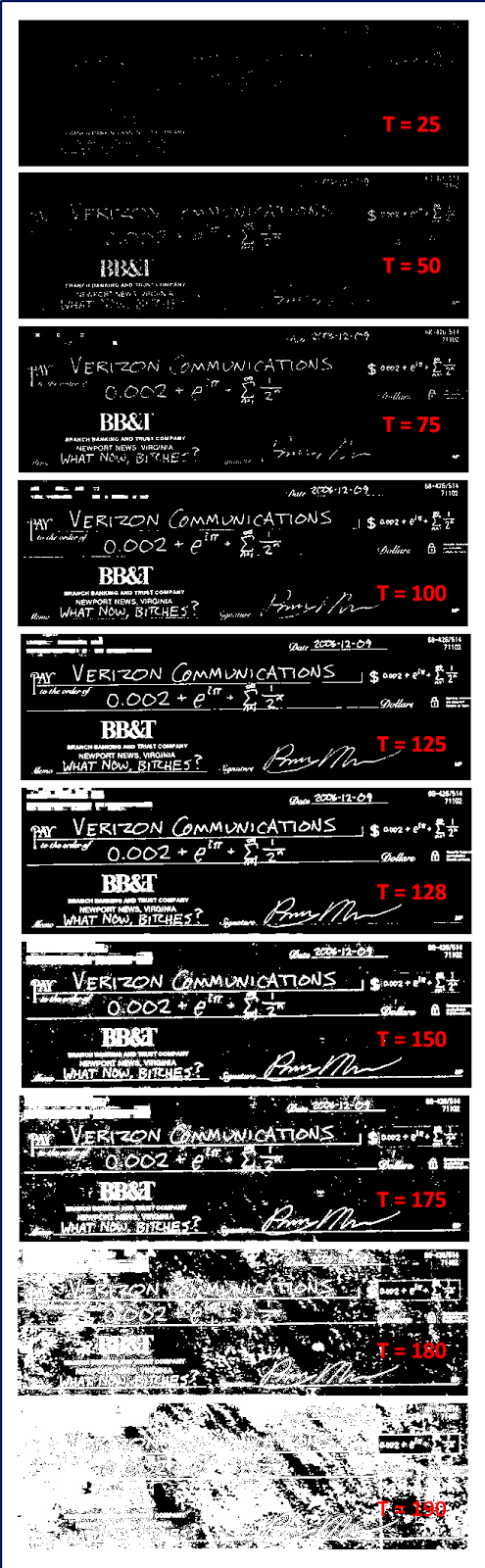
To determine how these operators work, we slice the image in Figure 12 into 256x256 subimages. We take the first subimage which is the first 256x256 slice at the topleft corner of Circles002.jpg. To separate the foreground from the background, we use the method of thresholding aided by a graylevel histogram as shown in Figure 13. We see that the appropriate threshold value is ~210 or 0.8235 if we use the im2bw() function.

Figure 13. Graylevel histogram of a subimage

As said earlier, binarizing an image may result to artifacts as seen in Figure 14: white areas on the upper edge and white dots can be seen on areas where we expect it to be black or zero. Since we are only interested with the white circles, we want to remove these artifacts.

Figure 14. 256x256 subimage considered from the top left portion of the iamge

In order to do that, we test out the operators as seen Figure 15.

Figure 15. a) Subimage operated with different morphological operators:(b) Closing (c) Opening (d) Black Tophat (e) White Tophat

Below is a simple description of what the respective operators do:

1. Closing operator = CloseImage(subbw,struc) =  erode(dilate(subbw,struc))

2. Opening operator = OpenImage(subbw,struc) = dilate(erode(subbw,struc))

3. White Tophat operator = subbw - OpenImage(subbw,struc)

4. Black Tophat operator = CloseImage(subbw, struc) - subbw

As we can see the Opening operator was successful in removing the artifacts and isolating the circles. In the IPD package of Scilab, one may use the function SearchBlobs() to label each aggregate of 1's in an image. This function aids us determine the area of each aggregate where the area refers to the sum of all ones.

Figure 16. Searchblobs function labels each blob of white pixels for easier analysis

Using the function, we take the area values of all the blobs in the subimages by scanning through all the aggregates from i = 1: max(Searchblobs(bw)) and plot its histogram.  

Figure 17. Histogram of areas in the subimages

From this distribution, we can get the mean and standard value of the areas in the images. It was found that the mean $\mu = 643.15$ and the standard deviation $\sigma = 455.39$. From these values, we can determine circles which are abnormal by filtering the areas above the sum of the mean and standard deviation.

Now we know about structuring elements and what the operators do. We also know the properties of the SearchBlobs() function. It's time to apply what we know to something practical with very much importance--the identification of cancer cells.

Figure 18 shows white circles with several larger circles which we identify as cancer cells. We want to filter these cancer cells using the techniques we learned earlier in the activity.

Figure 18. Circles with cancer cells.jpg

Below shows the binarized image and the identified blobs with areas exceeding the Threshold = mean(area) + stdev(area) with the use of the function in IPD, FilterBySize(bwlabel,Threshold) where bwlabel = SearchBlobs(bw). The function removes all the cells whose areas are below the threshold. The ones whose areas are above it are deemed abnormal. But as we shall see, because of the opening operator which erodes and then dilates causing the circles to get connected, aggregates are formed by normal cells which are retained by the FilterBySize() function. The next thing we need to do then is to separate these normal cells. Maam Jing suggested the use of Watershed Segmentation technique which you can read and learn using this tutorial: IPD Tutorial.

Figure 20. a)Binarized image b) Identified cells with area larger than the sum of mean and standard deviation c) Same with that in (b) but now we manipulate the graylevel value to see them easily

In class, I was doing the watershed segmentation part but luckily, because Maam Jing is doing her rounds, I was able to consult her about something simple that I did which automatically isolated the cells! I was very skeptic at first because the motivation that's in my head during the activity is to learn how to automate. Things like cancer are serious and needs fast action. Human error is not forgivable when lives are at stake. (Huuu I remember my med dreams but no.. I'm fineeee :)).

Well, back to the simple something. Remember, in the earlier part, I said something about the structuring element being important to get the desired result? Well, I proved its importance very quickly by using a circle as my structuring element whose radius is $r=15$. And tadddaaaa! I was able to get all five of them unlike the prior method that I used which only retained 3 out of 5! I was of course, pretty skeptic at first, but according to Maam Jing,the method which requires the least user input is already fine. So there, I have it. Yey! The identification of the cancer cells was a success!

Figure 19. Image with the identified cancer cells

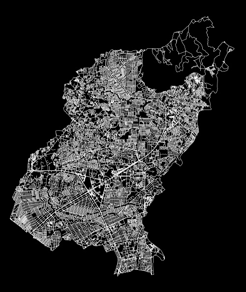
Now that I'm done with my activity, I can now go and explore. :D One quick thing that came to my mind while I was doing the activity is to apply morphological operations on my research. My research is on cities and I take interest in roads which are a city's one of, if not the most long lasting element. In particular, I want to apply the morphological operations to obtain a road network which is purely composed of one-pixel-thick lines. This is because, as we know, roads may contain islands. In my shapefiles, these islands will be rendered as a space in between the lines or, roads maybe multi-lane so that its thickness contributes much to space-filling. One of the metrics that I'm using to characterize my cities is the fractal dimension, $f_D$. My goal is to count the white pixels that cover the entire length of roads and not taking into account the thickness so much because the thickness will inflate the number of pixels and may return a very big value for the $f_D$. This will probably give a wrong impression of over space-filling!

So there, considering a map image of Quezon City as seen in Figure 20. What I want to get is a road network that is purely composed of 1-pixel thick lines.

Figure 20. Map of Quezon City

Figure 20 is a resized version of the map I'm using in research so that some information might be lost due to a decrease in resolution.

Figure 21. Binary image of QC map

Zooming into Figure 21,we will see roads which has spaces in between them.

Now, I apply the closing operator, which as you may recall is equivalent to Closing =  ErodeImage(DilateImage(im,struc)) where the structuring element that I used is a 1x2 ones. I got the following result:

Figure 22. Resulting image using the closing operator with a 1x2 ones structuring element

The difference is not very obvious, but zooming in, we will see that the thin spaces in between have closed and that the road network is now composed of approximately purely lines.

I also found a morphological operator in Matlab, 'skel' which is a part of the bwmorph() function which maybe the more appropriate operator for my problem. 'Skel' removes the pixels  on the boundaries of objects but does not allow them to break apart. The remaining make up the image skeleton. 

References:

[1] M. Soriano, "Morphological Operations",AP 186 class manual.(2016)

[2] R. Fisher,S. Perkins,(2003) "Morphology", retrieved from http://homepages.inf.ed.ac.uk/rbf/HIPR2/morops.htm on 22 October 2016.

[3] P.Peterlin,"Morphological Operations: An Overview", retrieved from http://www.inf.u-      szeged.hu/ssip/1996/morpho/morphology.html on 22 October 2016

Activity 7: Image Segmentation

Image segmentation is the process of partitioning an image into multiple regions with the aim of making the image easier to analyze.  It includes detecting the boundaries between the objects in the image. A good segmentation can be: 1) pixels belonging to the same category have the same grayscale values and form a connected region; 2) Adjacent pixels that do not belong to the same category hasve different multivariate values. In this activity, we look into two types of image segmentation, thresholding and region-based segmentation.

Image segmentation is a critical step in image analysis. The subsequent steps become a lot simpler when the parts of the image have been well identified.

The first step is to identify a region of interest (ROI) which contains characteristics that are unique to it. This ROI will serve as a reference to categorize the pixels in an image.

In grayscale images, segmentation is done via the process of thresholding. It is the simplest and most common method of segmentation. In this method, the pixels are allocated according to the range of values in which the pixels lie.

Consider Figure 1 which contains an image of a check. The goal is to recover the handwritten text.

Figure 1. Original image

Below is the code used to convert Figure 1 into a grayscale image and obtain its grayscale histogram.

Figure 2. Code to get grayscale histogram and to convert to BW image with different threshold values

Figure 3. Grayscale histogram of the input image in Figure 1.

Figure 3 shows the grayscale histogram of Figure 1. It gives us the number of pixels of a particular grayscale value. The peak corresponds to the background pixels. So the grayscale value of most of the pixels is around g~ 190.

In thresholding, the pixels are categorized into two i.e. black or white. Pixels whose grayvalue are below the threshold are classified into one category and those above are in the other category.  Here I tested different thresholds and see identified the value which will give me the clearest handwritten text.

\[ threshold \,T = 25,50,75,100,125,128,150,175,180,190\]

Figure 4. BW images with different threshold values

We will see that for T = 125 we can already recover the text. But knowing that the pixel value ranges from 0-255, I also tried out T = 128 which is basically T = 0.5 if we normalized the pixel values. It gave a slightly better result as we will not see any broken line in the image.

From the histogram in Figure 3, we will expect the result for T = 190. Since the peak corresponds to g = 190, it means that almost all of the pixels will be classified into the higher boundary i.e. white and thus, we can almost no longer see the details on the check.

Now we proceed to the region-based segmentation  wherein we apply two methods: 1) Parametric Method 2) Non-parametric/Back projection histogram method

PARAMETRIC METHOD
It is not all the time that thresholding is successful in segmenting an image. In this case, we take advantage of another property of an image -- color. The colors that we see are a ratio of the three primary colors: red, green, blue  or RGB. In reality, there is variation in the shade of an object's color. An example would be the effect of shadows on the brightness of the object's surface. To solve this, we represent the color space by the normalized chromaticity coordinates or NCC. This way, the separation of brightness and chromaticity is taken care of.

Figure 5. Normalized Chromaticity Coordinates

Figure 5 contains the NCC. The y-axis corresponds to g while the x-axis to r. Consider a pixel and let

\[\begin{equation}\label{ncc} I = R+G+B \end{equation}\]

then, the normalized coordinates are given by \[\begin{equation}\label{r}r = \frac{R}{R+G+B} = \frac{R}{I} \end{equation}\]

\[\begin{equation}\label{g}g= \frac{G}{R+G+B} = \frac{G}{I} \end{equation}\]

where \[r+g+b = 1\] so that \[b = 1-r-g\]

We have now simplified the color information into only two dimensions r and g. Know that they contain the color information while I takes care of the brightness information.

From Figure 5, x = 1 corresponds to pure red; y = 1 corresponds to a pure green; the origin to pure blue and point (0.33,0.33,0.33) to white. Later in the non-parametric method, we will see how the color values in the image are distributed in the NCC plane.

Segmentation using colors is done by determining the probability of that pixel to be in a particular color distribution or the PDF of the color. The PDF is obtained from the color histogram of the chosen ROI. The color distribution of the ROI serves as reference to the pixels. Now, because we have represented the information using r  and g,  the PDF is also a combination of the probability of these two. For example,

\[\begin{equation}\label{PDF} p(r) = \frac{1}{\sigma_r \sqrt{2\pi}}\exp{\frac{-(r-\mu_r)^2}{2\sigma_r^2}} \end{equation}\]

where the mean $\mu_r$ and standard deviation $\sigma_r$ are the parameters. The same can be done to find $p(g)$. The combined probability is the product $p(r)*p(g)$.

Now we consider the Santan flower in Figure 6 which will be the main object of interest and comparison for both methods of  region-based segmentation. What I want is to separate the flower from its background.

Figure 6. Santan flower

Notice that there is an obvious shade variation. Maam Jing has suggested for me to take samples of ROIs. Here I considered seven patches taken from the different regions of the Santan.

Figure 7. ROIs on the Santan flower

Below is the code to do the parametric segmentation.

Figure 8. Code used to do parametric method

Figure 9 shows the segmented images using the different ROIs. We will see that the sampling step is actually crucial. Patches 1-5 failed to fully separate the region of the flower. They look really nice thou! Looks dramatic. :) Patch 6 I think was most successful. Although the result of patch 7 looks really similar to that of patch 6, if one zooms into it, he will realize that it disregarded the small regions in between the flowers that do not correspond to the petals.Thus it did not really separate the regions.

The success of patch 6 I believe is due to the variation of colors and brightness in the patch itself. You may want to look at Figure 7 again for reference. The patch is taken from the center of one santan flowerette (if there's a name for the small flowers :) ).

Figure 9. Resulting segmented images using the parametric method

NON-PARAMETRIC METHOD AND BACK PROJECTION HISTOGRAM
We now proceed to the non-parametric method. By its name, we know that unlike the former, it is not dependent on any parameter like the mean $\mu$ and standard deviation $\sigma$ for computation and the separation process itself. Instead, the method is most dependent on the color histogram of the image.

Using the code given by Maam Jing in the manual, the 2D histogram was computed and eventually, we project this distribution into the actual image itself. The histogram will later then be compared to the NCC plane and see if it matches.

Figure 10. Code on the non-parametric method set-up and computation of 2D histogram

Figure 11. Back projection code

Figure 12. Resulting segmented images via the non-parametric method and their corresponding back projection histograms

Figrue 12 shows the results of the non-parametric method. The same can be said that patch 6 was most successful in separating the region of the flower. What surprised me though is the color distribution of the pixels. Though santan looks like coral-colored its color information says otherwise. It's in the blue and towards the green region.

The next important thing to do is to compare the results of both methods. For patches 1-5, the non-parametric method gave more desirable results since it gave more white regions that belong in the petal parts. But for patch 6 and 7 the parametric method was more effective since in the non-parametric, the regions which correspond to the in-betweens of the flowerettes are gone. So I guess, the parametric method can handle the finer details.

Figure 13. Comparison of the results of the Parametric [row 1] and Non-Parametric Method [row 2].

We have the theory and the code in our hands, it's time to have fun! This time I applied the methods to different images. Consider Figure 14 which contains my face and a crown of brown curly hair which will be my object of interest. 

Figure 14. My face and ROIs

Given the four ROIs, I want to separate my hair region from the rest of the image. The results were not nice. Scary,actually. Haha My facial region was also included! This could be because my hair is not dark and black. The gradient in the colors may not be too large. In the results, ROI #3's was the closest to being successful for both the methods since it separated my head from the background. But to compare, the parametric method is better since my face frame was also sort of separated from my crown of hair and details of my face are recovered too! :)

"Negative results are positive knowledge."    -Dr. M.Soriano (2016)

"Very timely and appropriate."- Me(right now)

Figure 15. Segmented images using both methods

Hours before I started working on the activity again, I was talking asking my friend about lipstick shades since my mom has been nagging me on my lack of talent in the field of beautifying myself. And since we're dealing with colors, I thought it would be interesting to look at lipstick colors more scientifically! Below is the palette of NYX lip balms launched in 2016. :)

Figure 16. NYX lip balm color palette

Figure 17, shows cropped parts which correpond to the ROI for each. The same methods were employed and what's left is to feed everything into the program.

Figure 17. Lip ROIs

The results are shown below. Looking at Figure 18 and 19 individually would seem as if both methods are tie in separating the respective lips for each ROI.

Figure 18. Segmentation via Parametric Method

Figure 19. Segmentation using Non-Parametric Method

Just a slight segue. Notice that the 2D histograms for all show the color distribution to be somewhere in blue-to-green regions. Even the Red Velvet and other seemingly shades of red. I believe that dark colors and pink shades [combination of red and blue] in general are found in this region. I also noted the result for the SuedeBerry which is a color very near to that of the Santan flower (only darker); the 2D histogram also looked similar.

Figure 20. Back projection histograms

Anyway,I opted to place them side-by-side and did some scoring with stars. Just like what teachers do in kindergarten! :)

Figure 21. Comparison of the two methods

This time, the non-parametric method emerged as the victor of segmentation with 11 stars! :)

What I deduced from the results is that, the parametric method is more efficient for images whose color gradients are not high or that the pixel rgI values are not very far away i.e. in the case of Santan and my picture whose differences lie on the shade. On the other hand, the non-parametric method is more appropriate for images which contain colors which differ obviously from each other such as the case of the NYX palette. But then again, since I only tested a few samples, this conclusion may be wrong.

Another thing that I explored in this activity is the effect of the size of ROI to the segmentation. I found out that the size matters but only very slightly. Resizing it but maintaining the aspect ratio won't have any effect at all.The key is in choosing the ROI such that it captures the range of colors in the entire region.

Rating: 10/10  because I did my best and had fun! :)

References:

[1] M. Soriano,"Image Segmentation", Class manual.(2014).

[2] "Chapter 4. Segmentation", retrieved from http://www.bioss.ac.uk/people/chris/ch4.pdf on 2 October 2016.