Activity 6: Properties and Applications of the 2D Fourier Transform

To give an easily imaginable picture of the FT, imagine your favorite food and you want to learn how to cook it. For you to do that, you have to know the recipe. FT is just the thing for you! Think of your food as a signal composed of many sinusoid components which in this case are the ingredients. The FT is a process that will decompose your favorite signal into its recipe. Basically, it answers the question of how much of this component sinusoid with frequency $f$ is in the signal?

In this activity, we explore the properties of the FT process.Note that since we are dealing with digital images, our FFT in this sense refers to the DFT. The DFT is a sampled FT in a particular interval and does not contain all frequencies but only a set of samples sufficient to describe the spatial domain. Images are easily obtainable 2D objects which makes them convenient to use as our object of study to explore the properties of the Fourier Transform.

A. Anamorphic Property of FT of Different 2D Patterns

From the previous posts, we knew that operations in the FT domain have a corresponding linear operation in other domains  (time and space) i.e. convolution:multiplication. Now we look into anamorphism, a property of the the FT domain wherein a large value (be it length) in one axis is small in another axis. To better explain this, it is best to look at the FT's of the following simple patterns. The patterns are generated through Scilab to ensure symmetry.

Figure 1. Narrow Rectangle with corresponding FT

Figure 2. Wide Rectangle with corresponding FT

Figure 3. Symmetric Dots, d = 0.5

Figure 4. Symmetric Dots with varying distances, d = 0.3 (top) and d = 0.7 (bottom) and their corresponding Fourier Transforms

Figures 1-4 exhibit the anamorphic property of FT. The narrow rectangle for example which is long along the y-direction in the spatial domain is short in the frequency domain. This time, the fourier transform is oriented largely along the x-direction. Anamorphism not only refers to the difference in the sizes along the axes in the different domains. Note that Figure 3 and 4 show that as the distance $d$ from the center along the horizontal becomes large, the grating spacing is small! The domains therefore have an inverse relationship with each other. We can also think of the distance in the spatial domain as the frequency of the sinusoid in the fourier plane.

B. Rotation Property of the FT

Figure 5. Corrugated Roof with $f = 4$ and its FT

This part seems to be the inverse of the previous [finding the FT of the two dots] only that the orientation is now along the y-direction.

As mentioned, the frequency of the sinusoid is proportional to the spacing of the dots in the fourier plane. We can treat the FT of these pairs as a series of interferograms of the signals with varying frequencies \[f = 4,8,16,20\] What if we're only given the signal itself? How do we determine the frequency? Well, what we can do is to take the distance of dot pairs from the central dot which is the brightest and take its average.

Figure 6. Corrugated roof with varying frequencies

Next, I added constant biases as seen in Figure 7. Figure 7a shows the original corrugated roof with $f = 4$ and no bias yet. Fig7b-7e are sinusoids of frequency $f = 4$ but with biases \[ bias = 0.2, 0.4, 0.6, 0.8\] Note that as we increase the value of the bias, the white portion widens and that the number of  dots in its corresponding fourier plane decreases. This could be because our viewing window is biased at a particular portion of the plane, which only allows us to see fewer frequencies.

Figure 7. Corrugated roof with added constant biases.

Figure 8 shows the corrugated roof with an added non-constant bias. The bias is in the form of a sinusoid with a very low frequency. As can be observed, there is now a non-uniformity  in the bright and dark regions and that its FT also differs. We can not observe white dots alone but thin elongated regions in its place.

Figure 8. Corrugated roof with added non-constant bias.

Now we rotate the sinusoid by $\theta = 30^{\circ}$.  Note that we have a signal that runs along the x and y. The addition of the rotation term does not in any way affect the intrinsic properties of the signal itself but only rotated its axes. We can see then that the FT of the corrugated roof are dots rotated by the same amount with respect to the x axis.

Figure 9. Corrugated Roof rotated by $\theta = 30^{\circ}$

On the other hand, Figure 10 is a sum of one sinusoid along the x-direction and another sinusoid along the y-direction. What we got resembles a checkerboard as can be seen below. Since the signal intersects repeatedly in the spatial domain, we expect the same repetitive pattern in the frequecy domain. Thus its FT resembles a weave pattern which also describes its spatial counterpart.

Figure 10. Combination of sinusoids along the x and y direction

Figure 11. Combined and rotated sinusoids

Figure 11 shows a combination of sinusoids but at the same time is being rotated by $\theta = 50^{\circ}$. Note that the amplitude and frequency of the wave seem to differ. This could be because one of a sine and the other is cosine. The displayed modulus shows the expected rotated, repetitive pattern and seem to propagated more along the x in contrast to the one in its spatial counterpart which runs more along y. Remember the  anamorphic property?

C. Convolution Theorem Redux

In this part of the activity, we will look at the dirac delta and its convolution to some patterns and also their respective FTs.

Figure 12. Symmetric Dots and corresponding FT

Two dots are symmetrically spaced from the center by $d = 0.5\,units$ and its FT was obtained this time. I will no longer discuss this any further since it was done earlier in this activity. What I want to emphasize here then is that we can think of these dots as two dirac deltas located symmetrically from the center and that the following patterns replacing the dots are patterns convolved with the dirac delta themselves.

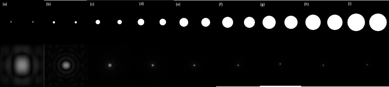
Figure 13. Symmetric Circles with varying radii

Figure 14. Symmetric Squares with varying widths

Figure 15. Symmetric Gaussian with varying variance values $\sigma$

Figures 13-15 show a circle, square and gaussian in place of the dots. For each pattern, an important parameter for each is varied and the behavior of its FT is noted. For example, for the circle we vary the radius $r$; the width $w$ for the square ;and the variance $\sigma^2$ for the gaussian. Note that as we increase the value of each parameter, the size of its counterpart in the fourier plane decreases. This is another display of the inverse property of the fourier pairs.  For the FTs of all the patterns: airy pattern for the circles; sinc function for the squares; and gaussian for the gaussian, we will observe the corrugated pattern in Figure 12. This pattern as we know is a sinusoid. For instance, the fourier of a square is a sinusoid.We can therefore say that the resulting FT is actually the FT of the convolution of the dirac delta and the function themselves!

Figure 16. Dirac delta simulated as white pixels distributed at random locations convolved with a 3x3 pattern "H"

Now we simulate 10 dirac deltas in space by scattering ten white dots randomly in space and a 3x3 pattern of "H" is convolved with it. You might already figured out that convolving any pattern with a dirac delta will only give the exact pattern but is located at the exact locations of the dirac. Note that the value of the white pixel is 1 and 0 otherwise. From primary school, we know that multiplying anything with zero gives us zero. So its like we're only multiplying the values on the planes and we're simply getting its product.

Figure 17. Dirac Delta with varying spacing

In Figure 17, we consider the dirac deltas spaced \[ s = 5,10,15,20,25\,pixels\]  away to be our signal and here we  observe anamorphism. The nearer the diracs in space, the farther they are in the fourier domain. Retaining the dots,  the FT of a dirac is then a constant.

D. Fingerprints: Ridge Enhancements

For the remaining parts of the activity, we make use of our knowledge of the properties of the 2D FT and apply it to image correction.

Below shows (a) my right thumb mark (b) its grayscale image and (c) its FT. It can be seen that the ridges of my thumb are not so well-defined. And that's the problem we want to address. From the FT of our original image, we can design a filter to remove the unwanted frequencies

Figure 18. Thumb mark

Common sensically, we know that what a filter does is to stop something from passing through. But still, I would like to emphasize that a filter never introduces new information. Figure 19 shows the filter I designed to enhance my thumb mark image. What do you think will happen?

Figure 19. FT of thumb mark and the designed filter

Figure 20 shows the enhanced thumb mark! :)

Figure 20. Enhanced thumb mark

To better appreciate it, we add contrast in the image making dark lines darker and light areas lighter by converting Figure 20 into its binary image counterpart.

Figure 21. Binary image for appreciation, threshold value = 0.5

E. Lunar Landing Scanned Images

This part seemed to be intimidating at first. To me, I felt like I was thrown off into the deep waters for the first time after teaching me the theory of swimming! I was only given the question and no directions this time. But when I come to think of it, this is how my research with my Ama (Dr. Batac) started. He posted a basic question and I'm answering it now in all the ways I know and I could.

Anyway, back to the problem at hand, we can see horizontal lines and we want to remove them.

Figure 22. Lunar crater

So we know that the filtering occurs at the fourier domain and thus the next obvious thing is to look at the image at that domain itself (Figure 23b).

Figure 23. Grayscale image and FT

Figure 24.Filtered image

What we want then is to remove the high frequency-signals but noting that information should still pass to recover the important ones and effectively the enhanced image. This time, my filter consists of vertical and horizontal lines along the axes but the center being kept open as to not lose the info. What we want is to remove the horizontal lines so by anamorphism, if its thick in one dimension, it should be thin at the other domain. Or you could think of the thickness as the degree of filtering.

Figure 25. Before and after

Figure 25 shows the original and the enhanced images which I deliberately placed side-by-side for comparison.


F. Canvas Weave Modeling and Removal

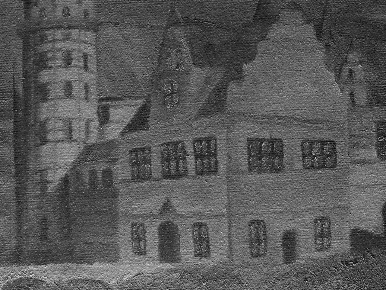
This part was the most challenging for me. I did this part alone for 5 to 7 days. :( The goal is to clean the image such that the weave patterns caused by the texture of the canvas itself is removed.

Figure 26. House

Figure 27. Grayscale of the original image

Figure 28. FT of the original image

Ironically, the filter that I ended up using is actually a very simple one drawn from very simplistic thinking. It consists of black circles which block the white spots or the peaks in the FT of my image. I retained the center peak which is the DC as to not filter all the information.

Figure 29. Filter used

Now I have my desired result! It now looks like a charcoal or pencil work. The surface looks smooth.

Figure 30. Cleaned Image

To know what information and how much I filtered, I took the complement of my filter and convolved it with the FT. Figure 32 shows the filtered information.

Figure 31. Complement of the filter

Figure 32. Filtered information

As I said earlier, I did this part for so many days I tried so many filters, mostly made manually. The following shows some of my test filters and their corresponding enhanced image; the filter complement; and the lost information. Because I'm a simple kid, my instant intuition is to block the significantly large white portions with shapes that I think would best cover it up. What I did wrong was that, I also removed the central DC which also removed most of the information and thus the dark images in the second row and it is supported by the images in the fourth row of Figure 33.

Figure 33. Other filters tested and corresponding cleaned images and filtered information

Because I realized that mistake, now I tried an approach where I did not block the center by using a Gaussin with different \[\sigma^{2} = 0.1,10,50,100\]They look better don't they especially the last column? But zooming in, because the method is just the inverse of the one I did previously, the result is also just the opposite of it: This time, too much information passed through the filter! One will realize this if he zooms-in. The enhanced images still contain weave patterns on their surface but to a lesser degree. But because the ratio of the white to black is not very large, we can still recover the image of the house in the images in the fourth row which correspond to the lost information except of course for the first column which actually just recovered the gray image and not much information was lost.

Figure 34. Gaussian filters with different variances

Rating : 10/10 because I was so bothered by the problem I dreamed of this activity for the entire week that I lost sleep.

Acknowledgements:

I want to express my gratitude to the following people:

Nina Zambale for the first part. She was sharing to me how she did things. Made Parts A-B easier! :D

Carlo Solibet because mostly, he's the one I can talk to about these things. :) So I consult him every now and then even with laptop troubles because we have the same laptop we both encountered stacksize error. He was also very patient when I'm becoming sabaw.

Angelo Rillera same with Carlo. I consulted him most especially on the filter-making. Kudos to Gelo for pausing on his blogging to help me debug my code for the filter! Very helpful and patient to those in need! Pagpalain ka.

Patrick Elegado and Micholo Medrana for also helping me debug my code for the filter.

References:

M. Soriano, "Properties and Applications of the 2D Fourier Transform", class manual. (2016)

Activity 5: Fourier Transform Model of Image Formation

Fourier Transform (FT) decomposes a signal into its component frequencies. This process "transfers" us into the frequency domain from  any physical domain of a signal i.e time and space domain. FT gives a complex-valued function of frequencies whose the absolute value indicates the magnitude of a given frequency and the  complex argument indicates the offset on the signal phase.

 The Fourier Transform of a signal is given by the integral

\[\begin{equation} \label{eqn:FT} F(f_x, f_y) = \int \int f(x,y) exp(- i 2\pi (f_{x}x + f_{y}y)) dx dy \end{equation} \].

where $f_x$ and $f_y$ are its frequencies along the orthogonal directions.

In this activity, we explore the FT and its operations and its uses in image processing.

For the first part, we got to familiarize ourselves with the Fast Fourier Transform (FFT) algorithm which was developed by Cooley and Tukey. FFT computes for the Discrete Fourier Transform or DFT which converts a finite-sequenced signal whose samples are equally spaced into a sequence of complex value function of frequency with equivalent length. The Cooley-Tukey algorithm recursively breaks down a DFT of composite size \(N = N_1N_2\) into smaller DFTs. Sounds complicated. Luckily, Scilab has functions fft2() and fftshift() which interchanges the quadrants of the signal and back respectively.

 Using the knowledge I acquired from Activity 3, I created a 128x128 image of a circular aperture whose radius \(r = 0.1\).(Note: The size is consistent for all the images used in this entry since FFT algo works best for images whose dimension are in powers of 2.)

Figure 1. Circular aperture with r = 0.1

Fig.1 which shows a circle centered at the origin with \( r = 0.1\) was used as our first test object. We apply FFT on the image and later the inverse to recover the original image using the code below.

Figure 2. FFT Code

After reading the image using imread, we FFT-ed the image using  the function ff2(). Since imshow() can only show 8-bit grayscale images,we included an extra step (Line 16 of the code in Fig. 2)  for us to be able to display the resulting images.

Figure 3. a) Input image b) FT of image c) FT shifted d) Inverse FT

Fig. 3 shows the  (a) input image and the (b)-(d) resulting patterns after it has undergone the process of Fourier transform. As seen FT interchanges the quadrants along the diagonals as seen in Fig 3b and the fftshift() function interchanges them back as seen in Fig.3c. Also in 3c) we note that the FT of the input circle results into concentric circles with varying intensity that seem to radiate from the center (which has the greatest intensity). In optics, for a lens system, these concentric circles represent interference patterns. Applying the inverse FT only returned the original image as seen in Fig.3d. The inverse FT is expected to give an inverted image of the original but since the circle is symmetric in both directions, we seem to recover the input image. Since we know that the FT returns a complex-value function, we display its real and imaginary components.

Fig.4 shows the real and imaginary components of our input image which is the circle. Notice that the real part resembles the FFT of the input. On the other hand, the imaginary part seem to be a zoomed-in version of it only that, there is a discontinuity across it.

Figure 7. Real part (L)  and Imaginary part (R) of the cirlce.

Since the circle is a symmetric object, we did not exactly see the expected effect of the inverse FT. Now, we apply the same process (as done in the code in Fig.2) to the letter "A" as the aperture.

Figure 5. Letter A.

Below are the results.

Figure 6. a) Input image b) FT of image c) FT shifted d) Inverse FT

Notice that the FT of the image in Fig.6c displays symmetry along the x-direction. I suppose that the observed symmetry for any input image is dependent on the shape of the object itself given we are looking at it in the spatial domain. Also, we now see that the inverse FT recovers the original input image only that it is inverted. Similar to the circle, we also took the real and imaginary components of the letter A.

Figure 7. Real part (L) and Imaginary part(R) of "A"

As noted earlier, the FFT returns a complex-valued function which means it is composed of real and imaginary parts. The image that we see is the composite of the magnitude and phase of different frequencies. For the letter "A" the real part also resembled the FFT of the original image. It is symmetric along the x and y direction. Moreover, the imaginary part as seen in Fig.7(R), looks like a close up version of the imaginary part.

We also applied the FT to other patterns namely a)Corrugated Roof b)Simulated Double Slit c)Square Function and d)2D Gaussian Bell. For all these patterns, we only applied the fft2() and fftshift() functions since the double fft2(fft2(image)) will only give us the inverted input. These patterns will serve as optical apertures (Fig8a - 11a)  and we will find out the resulting patterns (Fig8c-11c) as light passes through them. We will not give much focus on Fig.Xb since the patterns are unclear and are found almost at the edge as indicated by the red arrows.

Figure 8. Corrugated Roof

Fig.8c shows white dots whose intensity diminishes as it goes farther away from the middle. We could think of it this way: A coherent monochromatic light source is positioned orthogonal to the corrugated aperture. As light hits on the slopes for the side slits, light is diminished as interference happens and the one in the middle remains focused.

Figure 9. Simulated Double Slit

We recover the interference pattern observed in the Double Slit experiment. It is not very clear, but Fig.9b shows a repetitive pattern along the horizontal. What's not seen are the ones along the bottom part of the image. The simulated double slit aperture was succesful in producing the expected interference patterns.

Figure 10. Square Function

Just like in the first part of this activity, we observed concentricity for the square function aperture (Fig.10). We see lines radiate from a point along the x and y directions. If we zoom-in into Fig.10c, we will realize that the white spot is square in shape only that the edges seem to be smeared.

Figure 11. 2D Gaussian Bell

Lastly, we consider a 2D Gaussian bell aperture. One obvious characteristic of the gaussian bell is that it is most intense in the middle and slowly transitions to lower values ($\rightarrow 0$) as it goes away from the center. If we look closer at Fig.11c (encircled with red broken lines) we will see that after applying FT, we get a white dot in the middle. The interference patterns are no longer observable! No surprise, we know that the highest pixel value is found in the middle such that if we find apply the abs() function which gives us the magnitude, it will give us the point with highest value only.

Linear operations in one domain e.g. time domain has a corresponding operation in the other domain i.e. frequency domain and vice versa. One such operation is convolution which is basically the distortion of a function to conform to the form of another function such that the resulting function looks a little like both.

\[\begin{equation} \label{eqn:convolution} h(x,y) = \int \int f(x', y')g(x-x', y-y')dx' dy'\end{equation} \]

where $h(x,y)$ is the convoluted resulting function of two 2D-functions $f$ and $g$.

\[\begin{equation} \label{eqn:convolution2} h = f*g \end{equation}\].

As seen in Eqn. 3, (the shorthand expression for Eqn.2) convolution is done by simply multiplying the two functions. Consider Figure 12, a monochrome logo of the acronym "VIP" in bitmap format as one function, say $f(x,y)$ and is our input object. Whatt we want to do for this section is to see what happens if we make "VIP" pass through a circular aperture which we consider to be an imaging device or a black box. Let the aperture be $g(x,y)$. Figure 13 shows the results of the convolution between the two for varying aperture radii $r = [0.025,0.05,0.1,0.3,0.5,0.7,0.9]$. 

Figure 12."VIP" in monochrome bmp. format

By the way, here is the code I used for convolution.

Figure 13. Code used to find convolution

Figure 14. Circular apertures of varying radius and resulting convoluted images.

The effect of the aperture size is apparent as seen in Figure 14. As the radius is increased, the resulting image becomes more defined as we would expect on the actual setting. The bigger the aperture of the camera, more light comes in resulting into a better photo.

Figure 15. Spatial functions $f$ and $g$ we want to correlate

Another operation that we could do on two spatial functions $f(x,y)$ and $g(x,y)$ is to find their correlation  or the degree of similarity between them. Mathematically, correlation is defined as 

\[\begin{equation}\label{eqn: convolve}p(x,y) =\int \int f(x',y')g(x+x',y+y')dx' dy' \end{equation}\].

In a more practical perspective, this operation can be used in recognizing similar patterns in text or images and also in template matching. Consider the two images in Fig.15 two the functions $f$ and $g$ respectively. The goal is to find $g$ given as the letter A in $f$ which is the statement. 

To execute the process, here is the code:

Figure 16. Code to find correlation

Figure 17. Main text (L), Correlation result (M)  and mapped location of similar patterns in the text (R).

Fig.17(M) shows the correlation between the images in Fig.15.  The Fig.17b is a distorted chromatically inverted image of the original text in Fig.15(L) with five white spots whose intensity is relatively greater than its surroundings. By eye inspection, we could confirm their locations in Fig.17(L) by comparing it with the rightmost image.

Now that we are familiar with the process of fourier transform and convolution and correlation (with correlation looking similar to convolution only that we take the conjugate of one function), we explore another useful application that is a composite result of the three--edge detection. Using the same spatial function $f(x,y)$ (or the VIP logo), what we want is to detect its edges using a given matrix a) horizontal b) vertical c) diagonal d)spot e) random whose elements sum to zero. These matrices when converted into images themselves will act as another spatial function $g(x,y)$.

Figure 18. Edge detection code using different pattern matrices

Figure 19. Pattern matrices and resulting edge images

Recognize that the pattern is decided by the magnitude of the element. For instance, the horizontal pattern matrix (Fig.19a) has 2's lined up in the middle row and all the surrounding elements are -1. The same goes for the vertical (Fig.19b) and diagonal (Fig.19c) patterns.  Note that the edges that are best recovered has orientations corresponding to the matrix. Thus, for the horizontal pattern matrix, it recovered the horizontal lines (or pixels) in the "VIP" very well. The same goes for the vertical and diagonal (most especially in the letter V) which is basically two diagonal lines meeting at the center. The spot pattern matrix (Fig.19d) recovered all the edges nicely compared to the random matrix in Fig.19e which returned thicker yet ragged edges.

Figure 21 Non-zero matrix 

I was curious as to why the sum of the elements for edge-detection matrices should be  zero so I tried out a random non-zero matrix and I got the result in Fig.20. Right, a non-zero matrix would give considerable magnitude to each pixel value so that it shall recover the entire VIP logo. Haha, silly me!

I would like to acknowledge my classmate, Carlo Solibet for teaching me the function imwrite() in Scilab which would automatically save my images to my computer. It greatly took out a large portion of work! I used to take snapshots of my screen, transfer them to paint and save the image. :)) Now, I know better. And also, he has greatly helped me debug my code whenever I get weird looking plots.


References:

[1] M. Soriano, "Fourier Transform Model of Image Formation", Activity 5 Manual. (2016)