Activity 11: Basic Video Processing

This activity is the last of my Applied Physics 186 activities. Here, we try to apply all of the image processing techniques we've learned during the sem to a sequence of images that are played continuously more commonly known as a video to extract information like the position of a ball in time. 

Consider a simple mechanics problem shown below: A ball is released from one end of an inclined plane. Find a) Its position through time b) The acceleration due to gravity, $g$.

We need to isolate the ball using color segmentation. Vid.1 is a 5-second video we want to process. We take each frame as an image and try to isolate the ball by taking a patch on the surface of the tennis ball as our ROI and then apply Parametric Segmentation. To know about this said technique, you can revisit my Activity 7 here. 

After the parametric segmentation, there are still some other blobs we want to disregard completely. To do this, I did morphological operations to remove these blobs. First, label each blob using the SearchBlobs() function and then, try to filter each using FilterBySize(). The following video shows the isolated ball.

Below is the code I used to isolate the ball and compute for the centroid.

Now that we have one single blob to track, we find its position by calculating for its centroid. The centroid is the coordinates of the blob's center of mass in the image so that it is in x and y. The problem can be solved using polar coordinates for ease in computation but since the centroid for every frame is an ordered pair of (x,y) we first use cartesian coordinates and then convert into polar. The following images contain the schematic diagram of the problem and also the derivation of the important equations.

Figure 1. Schematic diagram with the origin at the top of the ramp. Polar and cartesian relations are also derived.

We consider the origin to be at the top of the ramp inclined at an angle $\alpha$ and has a length $s_{max}$. The relationship of the cartesian to polar quantities are also shown.

Figure 2. Energu relations for a hollow ball from which we derived the velocity $\dot s$ at the bottom of the incline

We consider the tennis ball to be a hollow sphere with a moment of inertia $I = \frac{2}{3}mr^2$ and that its motion includes rolling without slipping along the incline. From the energy relation which shows the conservation of energy where the potential energy is equal to the kinetic, we can derive its final speed $\dot s$.

Figure 3. We take the derivative  of the expression for the velocity $\dot s$ in Figure 2 to get the acceleration of the ball along the ramp and then use trigonometry to get the acceleration along the horizontal.

Figure 4. The position of the ball per frame is tracked and then plotted against time

Images were extracted from the video with rate of 25 frames/second. For each frame the position of the ball is extracted. But the pixel location plotted against time is meaningless so we need to convert it into real physical units. To do this, we compute for the calibration factor $C$ which determines the length covered by a pixel unit. Shown below is the computation.

$L_{actual} = 7 ft$

$end_1 = (828,35)$

$end_2 = (5,104)$

Since the length is oriented along the diagonal, we cannot simply subtract the coordinates like we did in Activity 2. To find the length of the incline, we employ the distance formula.

$L_{image} = end-to-end distance = \sqrt{(825-5)^2 + (5-104)^2} = 825.887 px$

7 ft. = 825.887 px

$(7ft.)\left(\frac{12 in.}{1 ft}\right)\left(\frac{2.54 cm.}{1 in.}\right)\left(\frac{1 m}{100 cm}\right) = 2.1336 \, m$

$C = \frac{2.1336 m}{825.887 px} = 2.58 \times 10^-3 \,  \frac{m}{px}$

And the incline is tilted at an angle of $\alpha = \arctan\left({\frac{|35- 104|}{|828-5|}}\right)= 4.79224 ^{\circ}$

Now we know that a pixel represents a distance of $2.58 \times 10^-3 \,  \frac{m}{px}$. The next thing we need to do is to multiply all the x-pixel coordinates with this factor to get the position and space and then plot this against time mutiplied to $\frac{1}{25}$ which represents the time per frame.

Figure 5 shows the plot of the balls position in time as extracted from the video frames. Now we can compare the coefficients of the fit with the theoretical as shown in Figure 4.

Figure 5. Position of ball in time with quadratic fit

We know that the concavity of the curve represents the acceleration $\ddot x$ of the ball so that, $\ddot x = 2a = \frac{3}{10}\,g\,\sin\alpha$. Isolating $g$, we get

$g = \frac{20\,a}{\sin 2\alpha}$ where a  is the coefficient of the quadratic fit in the experimental plot of the position vs. time shown in Figure 5. The calculated value for the acceleration due to gravity is $g = 9.961863 \frac{m}{s^2}$ which deviates from the theoretical value by $1.5 \%$.

This has been quite a culmination of the image processing skills I acquired for the entire sem and a refresher of my mechanics. For this activity, I will rate myself 11/10 since I was able to effectively apply image processing techniques and  accomplish my objectives completely. And also, I believe the images (Figure 1-4) used to illustrate the problem involved much effort in creating and also they're neat! :D

References:

[1] M. Soriano, "Basic Video Processing", AP186 class manual. (2016)

Activity 10. Enhancement via Histogram Manipulation

An image histogram represents the frequency distribution of pixel values in an image. It tells us about the spread of the colors in an image; take for example black (value = 0) and white (value = 1) for grayscale images. The image histogram is actually the (graylevel) probability  density function (PDF) of the image. In some cases, images are dark and low contrast due to low exposure and poor lighting conditions and a histogram represents this by having peaks clustered at lower values of the histogram.

In order enhance low quality images,their histograms are manipulated. This is done  by remapping the Cumulative Density Function or CDF of the poor image with new grayscale values from a desired CDF. Suppose the graylevels r of an image has a probability distribution function (PDF) given by $p_1(r)$ and  the cumulative distribution function is given by 

\[ \begin{equation} \label{cdf} T(r) = \int_{0}^{r} p_1 \, g \, dg \end{equation} \]

where g is a dummy variable.

We want to map the r's to a different set of graylevel z's such that the new image will have a CDF given by \[\begin{equation} \label{cdf2} G(z) = \int_{0}^{z} p_2(t)\,dt \end{equation}\] where $p_2(z)$ is the PDF of the transformed image and t is a dummy variable. 

Figure 1 best explains the steps to be taken.

Figure 1. Steps in altering the grayscale distribution. (1)From pixel grayscale, find CDF value.(2) Trace this value in the desired CDF. (3) Replace pixel value by grayscale value having this CDF value in desired CDF(4).

Now that we know the steps, consider a picture of me with my research ate, Anjali Tarun at the Dome of Light in Taiwan during the Physics Society of the Republic of China (PSROC) Annual Meeting. This was taken using a phone camera. Because the background is really bright, we non-bioluminiscent creatures looked super dark! 

Figure 2. Ate Banana and I at the Dome of Light

For this picture and others, I considered three desired CDFs namely linear, logarithmic and parabolic as shown in Figure 3. I considered the last two functions because the human eye, as we know, has nonlinear response (more specifically, it reacts logarithmically).

Figure 3. Desired CDFs (from L-R): Linear, Parabolic and Logarithmic

Below is the result for my first image after remapping the CDFs with the desired ones previously shown in Figure 3. 

Figure 4a is the grayscale image of Figure 2. Figure4b-4d are the enhanced images using the Linear, Logarithmic and Parabolic CDFs. Figures 4e-4h are their respective PDFs for us to see how the images have improved while Figures 4i-4l are the CDFs. The same layout is done for the other images considered.

Figure 4. Results for Figure 2. (a) Grayscale image of the picture we want to enhanced while (b)-(d) are the resulting enhanced images using linear, logarithmic and parabolic CDFs. The PDF for each enhanced image was also shown by (e)-(h) to see how it improved by the change in the spread of the pixel values while (i)-(l) are the corresponding CDFs we want to remap.

We shall see that visually, the linearly and parabolically enhanced images looked comparable with each other but upon seeing the enhanced PDFs we see that the pixel values looked more spread out and varied more evenly across using the linear function.

Now consider a quick selfie with my close friend Ace who went out making digma with traffic to come see because I said I was sad.(Felt blessed beyond measure for the people in my life like Ace <3 ) We didn't care about the lighting basta may selfie and so again, we looked darker so it's not Instagram-able. :((

Figure 5. Quick selfie with Ace

The same procedure is applied to Figure 5. And the results are shown in Figure 6.

Figure 6. The same procedure applied on Fig. 5. It looks as though the parabolic function has the same effect as the linear.

Similar to the previous result, it seems that the result for linear is comparable with the parabolic but upon closer inspection, we shall see that the result for the logarithmic seems to have over exposure patterns on the surface.

Enhancement via histogram manipulation is not limited to grayscale images. It can also be done on colored images like the one in Figure 2. In the rgb manipulation, we manipulate the intensity I of the image and what I got is shown in Figure 7.

Figure 7. Enhanced colored image via RGB manipulation

For comparison, I also used GIMP 2.0, an image processing software that serves many functions, to enhance Figure 2. I set the curve to be logarithmic and the result is Figure 8. 

Instant whitening happened to us! *O*

Figure 8. Enhanced via GIMP

For this activity, I give myself an 8.5/10

Acknowledgements:

Thank you Angelo Rillera  for the helpful discussions!

References:

M.Soriano, " Enhancement by Histogram Manipulation",AP 186 class manual.(2016)

Activity 9: Playing Notes by Image Processing

This activity is another venue to showcase the image processing skills we have acquired so far.The aim is to play music from a musical score sheet.

From the discussion in the manual, we learned that Scilab can sing using the following script. The frequency values assigned for each note can be found here: soundwave frequency.

                       Figure 1. Code to play a part of the song "Mary Had a Little Lamb"

For the application, I considered another nursery rhyme we are all familiar with-- the "London Bridge".Below is the musical score sheet of the song.

Figure 2. London Bridge

Since some parts in the sheet are unimportant to accomplish our aim, we do some preliminary steps to remove them i.e removal of texts such as the title, conversion to black and white, the time signature and the cleft. We do this by using a Closing operator on the black and white image with a horizontal line as the structuring element,

Figure 3. Result after using a closing operator and a horizontal structuring element

Notice, that we were not able to remove the staff or the five lines where the notes lie. This means  that we need to yet apply another morphological operation. This time we  use the Opening operator with a circle (r = 1.5) to remove the lines and the stems of the notes. And what I got is shown below.

Figure 4. Staff and stems removed

Now what we want is to get rid of the large blobs that are the chords which are actually notes that are simultaneously played. To do this, I filtered the blobs using the function FilterBySize() which removes blobs whose areas do not fall within the specified range.

Because the London Bridge is a song introduced to children at a very early stage in learning, it is expected to have a repetitive pattern for easy retention. Notice that the rows have similar notes only differing in the 4th and 8th measure. For convenience, I only considered the upper row.

Figure 5. The upper row of notes containing the 1st-4th measures

Now we have the image that we want to read. This is actually my first time to read a musical score. I did not really like my music classes back in elementary and high school. So this activity is already a challenge from the very beginning. But from what I understood, the most critical is to determine the position of the note on the staff. For beginners like me, I recommend checking out this website for some basic explanation: How to Read Sheet Music.

Remember the code that can make Scilab sing? Well, it actually contains majority of what we need to accomplish in this activity.The critical part is to determine the vertical position of the notes. To do this, we again label the blobs and find the coordinates of its centroid using the Centroid function in the IPD library and then we assign the sound wave frequency value to each note.

Below is a snippet of the code which determines the centroid coordinates, area of the blobs which takes care of the note count other than that of a quarter note which is the simplest case i.e. whole note which will come in handy later; and ends in saving the music produced.

Figure 6. Code which determines the y-position of the notes and the soundwave frequency values

To listen to the final product of all these processes, see "London Bridge" by Scilab.

Right now, I am trying out other songs with more complicated elements. Just to get a feeling of accomplishment, I put all of these here and the result of my said exploration are to follow. :)

This is the activity where I learned the most because I had to learn how to read a musical sheet for me to start. So I felt that I was really starting from scratch. Huuu sweetest feeling of success! <3 And for that I give myself a 10. :D

Acknowledgments:

In the final part of this activity, I was stuck because what I got was a continuous stream of sound and the London Bridge tune is hardly recovered. I would like to thank Roland Romero for helping me solve the problem by teaching me a way to concatenate to a list appropriate to my note function and eventually produced the desired tune! :)

References:

[1] M. Soriano, "Playing Notes by Image Processing", AP 186 class manual. (2016)

[2] "Physics of Music-Notes" retrieved from http://www.phy.mtu.edu/~suits/notefreqs.html on 4 November 2016

Activity 8: Morphological Operations

Morphology is the study of shape.Mathematical morphology is a process where we take in binary images and operate on them to improve the image before further processing or to extract information from the image. The process' language is the set theory such that morphological operators take a binary image and a structuring element (or kernel but the term is mostly used in convolution). A point is either in the pixel set such that it is part of the foreground or not such the pixel is part of the background. Because of this, set operations such as intersection, union, inclusion and complement are applied. For more information, one can look up Mathematical Morphology.

The structuring element consists only of 1's and don't care pixels or pixels we can ignore. It is shifted across the image and at every pixel of the image it is compared with the ones underneath.If the condition defined by the set operator are met(e.g. the set of pixels in the structuring element is a subset of the underlying image pixels), the pixel underneath the origin of the structuring element is set to a pre-defined value (0 or 1 for binary images).[2]

The desired resulting image is therefore heavily dependent on the structuring element used.

In this activity, we look at morphological operations on the following shapes in Figure 1 with structuring elements which followed. In the first part, we were asked to draw the results to maybe check if we got the concept right. Later on, Scilab can help us check if we did.

Figure 1. Shapes

Figure 2. Structure Elements

The morphological operations are combinations of the two most basic operations: Erosion and Dilation. 

Erosion denoted by an enclosed minus sign erodes the boundary of the foreground pixels which makes the area of the foreground smaller and the spaces in between become larger. Dilation denoted by an enclosed plus sign on the other hand, does the opposite which expands the foreground and diminishes the spaces in between.

Below are my drawings  and I opted to place them separately to maintain the size for easy viewing.

I. Erosion

The eroded part is indicated by the boxes with "-". In each structuring element, the origin is indicated by a dot since we are dealing with operations that are based on the set theory which is dependent on a reference point.

Figure 3. Erosion of 5x5 Square

Figure 4. Erosion of Triangle 

Figure 5. Erosion of 10x10 Hollow Square

Figure 6. Erosion of Plus Sign

II. Dilation

Dilated parts are indicated by the "+"

Figure 7. Dilation of Square and Triangle

Figure 8. Dilation of 10x10 Hollow Square

Figure 9. Dilation of Plus Sign

To see if I predicted the output correctly, erosion and dilation were performed in Scilab. Figure 10a-10b are the results for the erosion 5x5 square with the structuring elements in the following order: 2x2 ones, 1x2 ones, 2x1 ones, cross, and diagonal which is 2 boxes-long. The same is done with the others. Figure 10e-10i Erosion of a B=4, H=3 Triangle; Figure 10j-10n Erosion of 10x10 hollow square; and Figure 10o-10s. Erosion of plus sign. Figure 11 displays the results for dilation and obeys the same ordering.

Figure 10. Erosion of the shapes with the structure elements performed in Scilab

Figure 11. Dilation of the shapes with the structure elements performed in Scilab

Now that we know how erosion and dilation works on images, we look at the different morphological operators: Closing, Opening, Tophat (White and Black). There are instances that there is an overlap in the graylevel distribution of background that sometimes result to artifacts after segmentation and binarization. The aformentioned operators will help us solve this problem.

Figure 12. Circles002.jpg

To determine how these operators work, we slice the image in Figure 12 into 256x256 subimages. We take the first subimage which is the first 256x256 slice at the topleft corner of Circles002.jpg. To separate the foreground from the background, we use the method of thresholding aided by a graylevel histogram as shown in Figure 13. We see that the appropriate threshold value is ~210 or 0.8235 if we use the im2bw() function.

Figure 13. Graylevel histogram of a subimage

As said earlier, binarizing an image may result to artifacts as seen in Figure 14: white areas on the upper edge and white dots can be seen on areas where we expect it to be black or zero. Since we are only interested with the white circles, we want to remove these artifacts.

Figure 14. 256x256 subimage considered from the top left portion of the iamge

In order to do that, we test out the operators as seen Figure 15.

Figure 15. a) Subimage operated with different morphological operators:(b) Closing (c) Opening (d) Black Tophat (e) White Tophat

Below is a simple description of what the respective operators do:

1. Closing operator = CloseImage(subbw,struc) =  erode(dilate(subbw,struc))

2. Opening operator = OpenImage(subbw,struc) = dilate(erode(subbw,struc))

3. White Tophat operator = subbw - OpenImage(subbw,struc)

4. Black Tophat operator = CloseImage(subbw, struc) - subbw

As we can see the Opening operator was successful in removing the artifacts and isolating the circles. In the IPD package of Scilab, one may use the function SearchBlobs() to label each aggregate of 1's in an image. This function aids us determine the area of each aggregate where the area refers to the sum of all ones.

Figure 16. Searchblobs function labels each blob of white pixels for easier analysis

Using the function, we take the area values of all the blobs in the subimages by scanning through all the aggregates from i = 1: max(Searchblobs(bw)) and plot its histogram.  

Figure 17. Histogram of areas in the subimages

From this distribution, we can get the mean and standard value of the areas in the images. It was found that the mean $\mu = 643.15$ and the standard deviation $\sigma = 455.39$. From these values, we can determine circles which are abnormal by filtering the areas above the sum of the mean and standard deviation.

Now we know about structuring elements and what the operators do. We also know the properties of the SearchBlobs() function. It's time to apply what we know to something practical with very much importance--the identification of cancer cells.

Figure 18 shows white circles with several larger circles which we identify as cancer cells. We want to filter these cancer cells using the techniques we learned earlier in the activity.

Figure 18. Circles with cancer cells.jpg

Below shows the binarized image and the identified blobs with areas exceeding the Threshold = mean(area) + stdev(area) with the use of the function in IPD, FilterBySize(bwlabel,Threshold) where bwlabel = SearchBlobs(bw). The function removes all the cells whose areas are below the threshold. The ones whose areas are above it are deemed abnormal. But as we shall see, because of the opening operator which erodes and then dilates causing the circles to get connected, aggregates are formed by normal cells which are retained by the FilterBySize() function. The next thing we need to do then is to separate these normal cells. Maam Jing suggested the use of Watershed Segmentation technique which you can read and learn using this tutorial: IPD Tutorial.

Figure 20. a)Binarized image b) Identified cells with area larger than the sum of mean and standard deviation c) Same with that in (b) but now we manipulate the graylevel value to see them easily

In class, I was doing the watershed segmentation part but luckily, because Maam Jing is doing her rounds, I was able to consult her about something simple that I did which automatically isolated the cells! I was very skeptic at first because the motivation that's in my head during the activity is to learn how to automate. Things like cancer are serious and needs fast action. Human error is not forgivable when lives are at stake. (Huuu I remember my med dreams but no.. I'm fineeee :)).

Well, back to the simple something. Remember, in the earlier part, I said something about the structuring element being important to get the desired result? Well, I proved its importance very quickly by using a circle as my structuring element whose radius is $r=15$. And tadddaaaa! I was able to get all five of them unlike the prior method that I used which only retained 3 out of 5! I was of course, pretty skeptic at first, but according to Maam Jing,the method which requires the least user input is already fine. So there, I have it. Yey! The identification of the cancer cells was a success!

Figure 19. Image with the identified cancer cells

Now that I'm done with my activity, I can now go and explore. :D One quick thing that came to my mind while I was doing the activity is to apply morphological operations on my research. My research is on cities and I take interest in roads which are a city's one of, if not the most long lasting element. In particular, I want to apply the morphological operations to obtain a road network which is purely composed of one-pixel-thick lines. This is because, as we know, roads may contain islands. In my shapefiles, these islands will be rendered as a space in between the lines or, roads maybe multi-lane so that its thickness contributes much to space-filling. One of the metrics that I'm using to characterize my cities is the fractal dimension, $f_D$. My goal is to count the white pixels that cover the entire length of roads and not taking into account the thickness so much because the thickness will inflate the number of pixels and may return a very big value for the $f_D$. This will probably give a wrong impression of over space-filling!

So there, considering a map image of Quezon City as seen in Figure 20. What I want to get is a road network that is purely composed of 1-pixel thick lines.

Figure 20. Map of Quezon City

Figure 20 is a resized version of the map I'm using in research so that some information might be lost due to a decrease in resolution.

Figure 21. Binary image of QC map

Zooming into Figure 21,we will see roads which has spaces in between them.

Now, I apply the closing operator, which as you may recall is equivalent to Closing =  ErodeImage(DilateImage(im,struc)) where the structuring element that I used is a 1x2 ones. I got the following result:

Figure 22. Resulting image using the closing operator with a 1x2 ones structuring element

The difference is not very obvious, but zooming in, we will see that the thin spaces in between have closed and that the road network is now composed of approximately purely lines.

I also found a morphological operator in Matlab, 'skel' which is a part of the bwmorph() function which maybe the more appropriate operator for my problem. 'Skel' removes the pixels  on the boundaries of objects but does not allow them to break apart. The remaining make up the image skeleton. 

References:

[1] M. Soriano, "Morphological Operations",AP 186 class manual.(2016)

[2] R. Fisher,S. Perkins,(2003) "Morphology", retrieved from http://homepages.inf.ed.ac.uk/rbf/HIPR2/morops.htm on 22 October 2016.

[3] P.Peterlin,"Morphological Operations: An Overview", retrieved from http://www.inf.u-      szeged.hu/ssip/1996/morpho/morphology.html on 22 October 2016

Activity 7: Image Segmentation

Image segmentation is the process of partitioning an image into multiple regions with the aim of making the image easier to analyze.  It includes detecting the boundaries between the objects in the image. A good segmentation can be: 1) pixels belonging to the same category have the same grayscale values and form a connected region; 2) Adjacent pixels that do not belong to the same category hasve different multivariate values. In this activity, we look into two types of image segmentation, thresholding and region-based segmentation.

Image segmentation is a critical step in image analysis. The subsequent steps become a lot simpler when the parts of the image have been well identified.

The first step is to identify a region of interest (ROI) which contains characteristics that are unique to it. This ROI will serve as a reference to categorize the pixels in an image.

In grayscale images, segmentation is done via the process of thresholding. It is the simplest and most common method of segmentation. In this method, the pixels are allocated according to the range of values in which the pixels lie.

Consider Figure 1 which contains an image of a check. The goal is to recover the handwritten text.

Figure 1. Original image

Below is the code used to convert Figure 1 into a grayscale image and obtain its grayscale histogram.

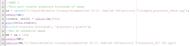
Figure 2. Code to get grayscale histogram and to convert to BW image with different threshold values

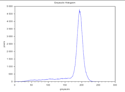
Figure 3. Grayscale histogram of the input image in Figure 1.

Figure 3 shows the grayscale histogram of Figure 1. It gives us the number of pixels of a particular grayscale value. The peak corresponds to the background pixels. So the grayscale value of most of the pixels is around g~ 190.

In thresholding, the pixels are categorized into two i.e. black or white. Pixels whose grayvalue are below the threshold are classified into one category and those above are in the other category.  Here I tested different thresholds and see identified the value which will give me the clearest handwritten text.

\[ threshold \,T = 25,50,75,100,125,128,150,175,180,190\]

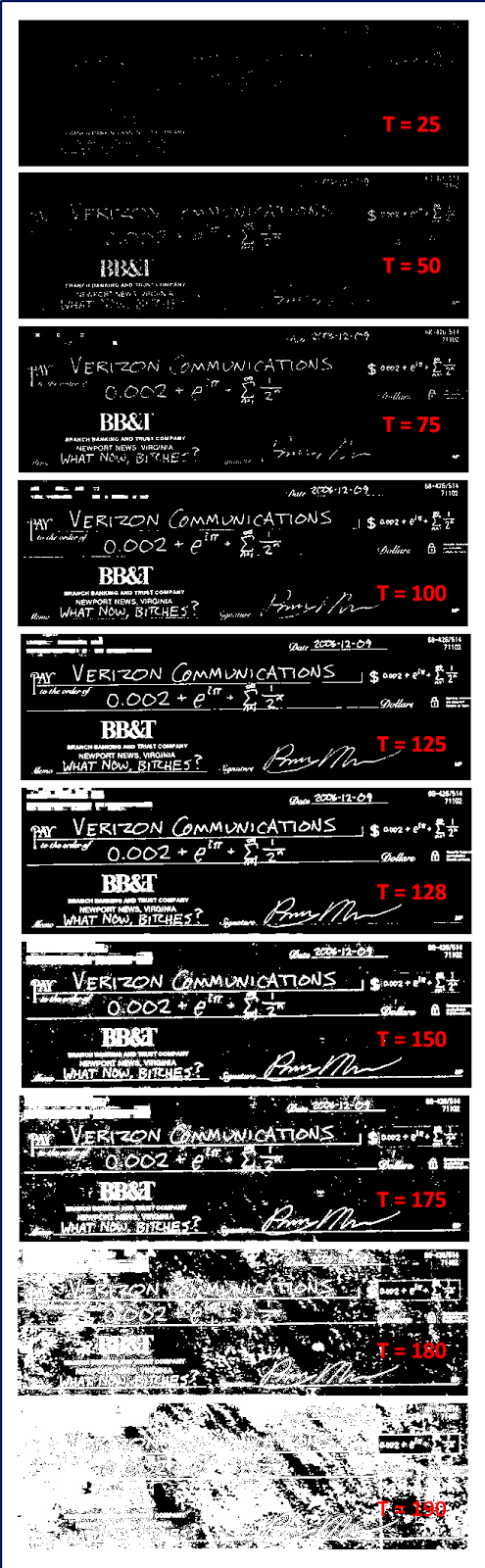
Figure 4. BW images with different threshold values

We will see that for T = 125 we can already recover the text. But knowing that the pixel value ranges from 0-255, I also tried out T = 128 which is basically T = 0.5 if we normalized the pixel values. It gave a slightly better result as we will not see any broken line in the image.

From the histogram in Figure 3, we will expect the result for T = 190. Since the peak corresponds to g = 190, it means that almost all of the pixels will be classified into the higher boundary i.e. white and thus, we can almost no longer see the details on the check.

Now we proceed to the region-based segmentation  wherein we apply two methods: 1) Parametric Method 2) Non-parametric/Back projection histogram method

PARAMETRIC METHOD
It is not all the time that thresholding is successful in segmenting an image. In this case, we take advantage of another property of an image -- color. The colors that we see are a ratio of the three primary colors: red, green, blue  or RGB. In reality, there is variation in the shade of an object's color. An example would be the effect of shadows on the brightness of the object's surface. To solve this, we represent the color space by the normalized chromaticity coordinates or NCC. This way, the separation of brightness and chromaticity is taken care of.

Figure 5. Normalized Chromaticity Coordinates

Figure 5 contains the NCC. The y-axis corresponds to g while the x-axis to r. Consider a pixel and let

\[\begin{equation}\label{ncc} I = R+G+B \end{equation}\]

then, the normalized coordinates are given by \[\begin{equation}\label{r}r = \frac{R}{R+G+B} = \frac{R}{I} \end{equation}\]

\[\begin{equation}\label{g}g= \frac{G}{R+G+B} = \frac{G}{I} \end{equation}\]

where \[r+g+b = 1\] so that \[b = 1-r-g\]

We have now simplified the color information into only two dimensions r and g. Know that they contain the color information while I takes care of the brightness information.

From Figure 5, x = 1 corresponds to pure red; y = 1 corresponds to a pure green; the origin to pure blue and point (0.33,0.33,0.33) to white. Later in the non-parametric method, we will see how the color values in the image are distributed in the NCC plane.

Segmentation using colors is done by determining the probability of that pixel to be in a particular color distribution or the PDF of the color. The PDF is obtained from the color histogram of the chosen ROI. The color distribution of the ROI serves as reference to the pixels. Now, because we have represented the information using r  and g,  the PDF is also a combination of the probability of these two. For example,

\[\begin{equation}\label{PDF} p(r) = \frac{1}{\sigma_r \sqrt{2\pi}}\exp{\frac{-(r-\mu_r)^2}{2\sigma_r^2}} \end{equation}\]

where the mean $\mu_r$ and standard deviation $\sigma_r$ are the parameters. The same can be done to find $p(g)$. The combined probability is the product $p(r)*p(g)$.

Now we consider the Santan flower in Figure 6 which will be the main object of interest and comparison for both methods of  region-based segmentation. What I want is to separate the flower from its background.

Figure 6. Santan flower

Notice that there is an obvious shade variation. Maam Jing has suggested for me to take samples of ROIs. Here I considered seven patches taken from the different regions of the Santan.

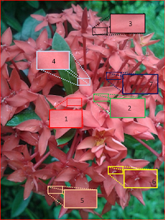
Figure 7. ROIs on the Santan flower

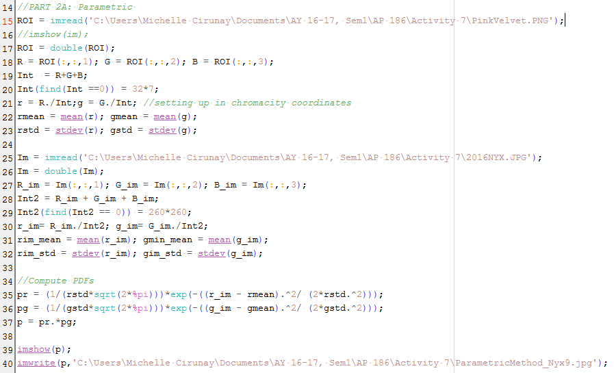
Below is the code to do the parametric segmentation.

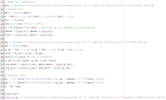
Figure 8. Code used to do parametric method

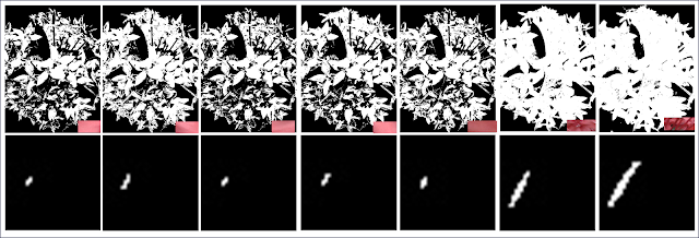
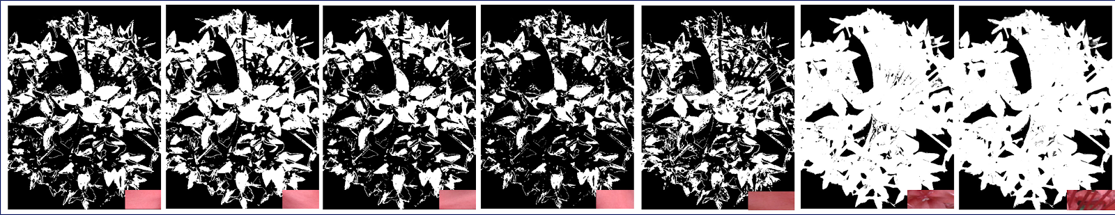
Figure 9 shows the segmented images using the different ROIs. We will see that the sampling step is actually crucial. Patches 1-5 failed to fully separate the region of the flower. They look really nice thou! Looks dramatic. :) Patch 6 I think was most successful. Although the result of patch 7 looks really similar to that of patch 6, if one zooms into it, he will realize that it disregarded the small regions in between the flowers that do not correspond to the petals.Thus it did not really separate the regions.

The success of patch 6 I believe is due to the variation of colors and brightness in the patch itself. You may want to look at Figure 7 again for reference. The patch is taken from the center of one santan flowerette (if there's a name for the small flowers :) ).

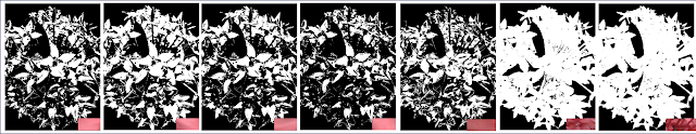
Figure 9. Resulting segmented images using the parametric method

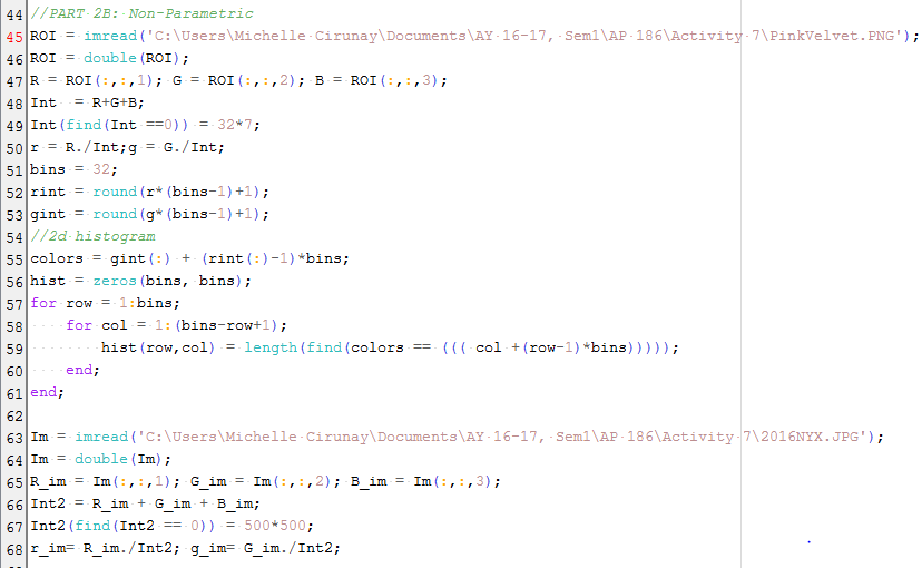
NON-PARAMETRIC METHOD AND BACK PROJECTION HISTOGRAM
We now proceed to the non-parametric method. By its name, we know that unlike the former, it is not dependent on any parameter like the mean $\mu$ and standard deviation $\sigma$ for computation and the separation process itself. Instead, the method is most dependent on the color histogram of the image.

Using the code given by Maam Jing in the manual, the 2D histogram was computed and eventually, we project this distribution into the actual image itself. The histogram will later then be compared to the NCC plane and see if it matches.

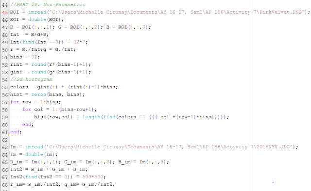
Figure 10. Code on the non-parametric method set-up and computation of 2D histogram

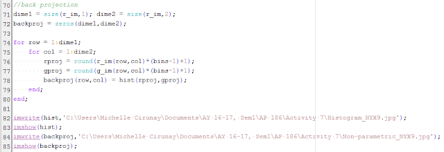
Figure 11. Back projection code

Figure 12. Resulting segmented images via the non-parametric method and their corresponding back projection histograms

Figrue 12 shows the results of the non-parametric method. The same can be said that patch 6 was most successful in separating the region of the flower. What surprised me though is the color distribution of the pixels. Though santan looks like coral-colored its color information says otherwise. It's in the blue and towards the green region.

The next important thing to do is to compare the results of both methods. For patches 1-5, the non-parametric method gave more desirable results since it gave more white regions that belong in the petal parts. But for patch 6 and 7 the parametric method was more effective since in the non-parametric, the regions which correspond to the in-betweens of the flowerettes are gone. So I guess, the parametric method can handle the finer details.

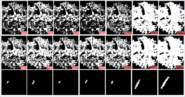
Figure 13. Comparison of the results of the Parametric [row 1] and Non-Parametric Method [row 2].

We have the theory and the code in our hands, it's time to have fun! This time I applied the methods to different images. Consider Figure 14 which contains my face and a crown of brown curly hair which will be my object of interest. 

Figure 14. My face and ROIs

Given the four ROIs, I want to separate my hair region from the rest of the image. The results were not nice. Scary,actually. Haha My facial region was also included! This could be because my hair is not dark and black. The gradient in the colors may not be too large. In the results, ROI #3's was the closest to being successful for both the methods since it separated my head from the background. But to compare, the parametric method is better since my face frame was also sort of separated from my crown of hair and details of my face are recovered too! :)

"Negative results are positive knowledge."    -Dr. M.Soriano (2016)

"Very timely and appropriate."- Me(right now)

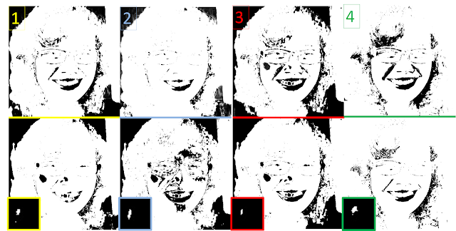
Figure 15. Segmented images using both methods

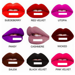
Hours before I started working on the activity again, I was talking asking my friend about lipstick shades since my mom has been nagging me on my lack of talent in the field of beautifying myself. And since we're dealing with colors, I thought it would be interesting to look at lipstick colors more scientifically! Below is the palette of NYX lip balms launched in 2016. :)

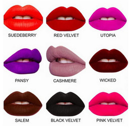
Figure 16. NYX lip balm color palette

Figure 17, shows cropped parts which correpond to the ROI for each. The same methods were employed and what's left is to feed everything into the program.

Figure 17. Lip ROIs

The results are shown below. Looking at Figure 18 and 19 individually would seem as if both methods are tie in separating the respective lips for each ROI.

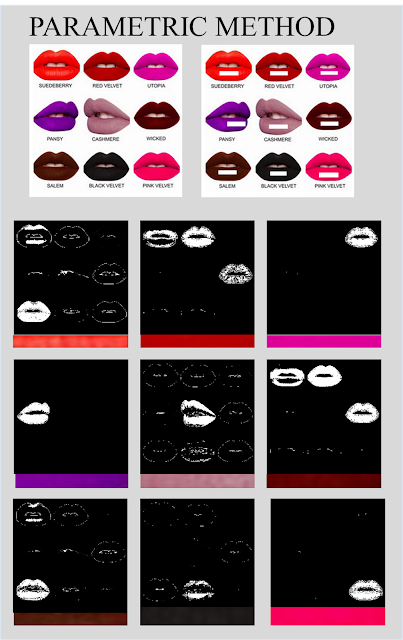
Figure 18. Segmentation via Parametric Method

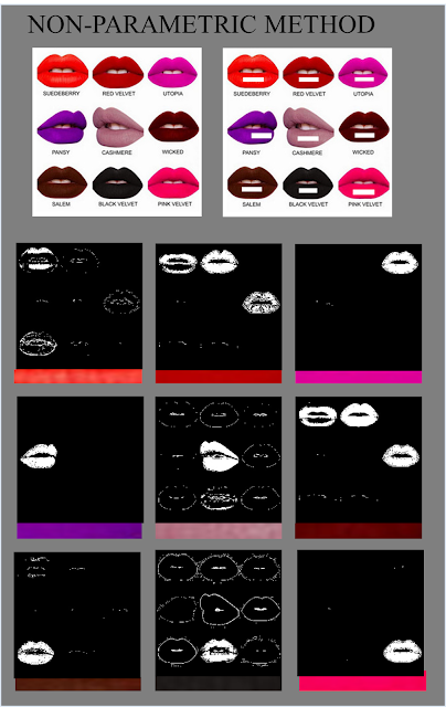
Figure 19. Segmentation using Non-Parametric Method

Just a slight segue. Notice that the 2D histograms for all show the color distribution to be somewhere in blue-to-green regions. Even the Red Velvet and other seemingly shades of red. I believe that dark colors and pink shades [combination of red and blue] in general are found in this region. I also noted the result for the SuedeBerry which is a color very near to that of the Santan flower (only darker); the 2D histogram also looked similar.

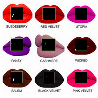
Figure 20. Back projection histograms

Anyway,I opted to place them side-by-side and did some scoring with stars. Just like what teachers do in kindergarten! :)

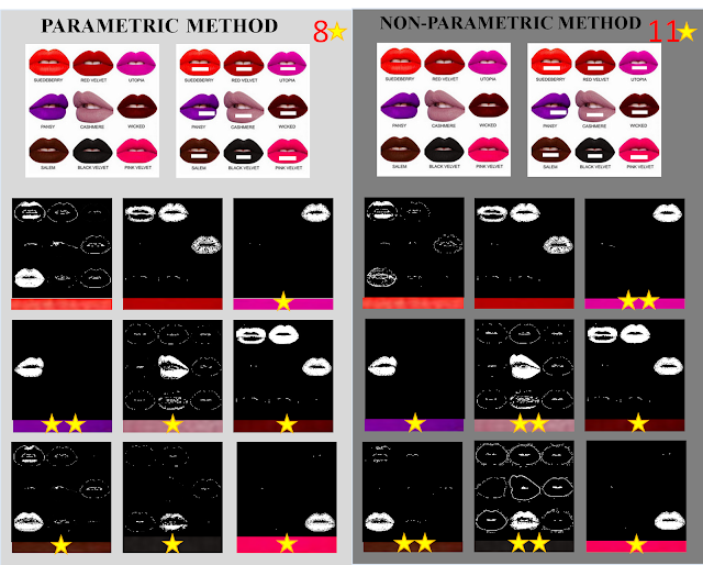
Figure 21. Comparison of the two methods

This time, the non-parametric method emerged as the victor of segmentation with 11 stars! :)

What I deduced from the results is that, the parametric method is more efficient for images whose color gradients are not high or that the pixel rgI values are not very far away i.e. in the case of Santan and my picture whose differences lie on the shade. On the other hand, the non-parametric method is more appropriate for images which contain colors which differ obviously from each other such as the case of the NYX palette. But then again, since I only tested a few samples, this conclusion may be wrong.

Another thing that I explored in this activity is the effect of the size of ROI to the segmentation. I found out that the size matters but only very slightly. Resizing it but maintaining the aspect ratio won't have any effect at all.The key is in choosing the ROI such that it captures the range of colors in the entire region.

Rating: 10/10  because I did my best and had fun! :)

References:

[1] M. Soriano,"Image Segmentation", Class manual.(2014).

[2] "Chapter 4. Segmentation", retrieved from http://www.bioss.ac.uk/people/chris/ch4.pdf on 2 October 2016.